728x90
▷ 1차원 연속형 확률변수
- 연속형 확률변수
- 확률변수가 취할 수 있는 값이 연속적인 확률변수
- 특정 값을 취하는 확률은 정의되지 않음
- 확률변수가 어느 구간에 들어가는 확률을 정의
- 확률밀도함수
- 확률변수가 취할 수 있는 값은 구간 [a,b]
- 확률은 확률밀도함수(PDF) 또는 밀도함수 f(x)에 의해 정의
- 어떤 특정 값을 취하는 확률로는 정의되지 않음
- f(x) ≠ P(X=x)
import numpy as np
import matplotlib.pyplot as plt
from scipy import integrate
import warnings
warnings.filterwarnings('ignore',category=integrate.IntegrationWarning)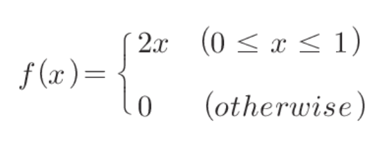
- f(x)의 확률밀도 함수 구하기
x_range = np.array([0,1])

def f(x):
    if x_range[0] <= x <= x_range[1]:
        return 2 * x
    else:
        return 0

X = [x_range,f]
X
- 확률밀도함수 그래프 그리기
plt.rcParams['axes.unicode_minus']=False
# (-) 값 깨질 시 True False 를 바꿔주면됨. (-)값만 해댱됨.

xs = np.linspace(x_range[0], x_range[1], 100)
# linspace : 100개를 균등하게 나눔.
fig = plt.figure(figsize=(10,6))
ax = fig.add_subplot(111)

ax.plot(xs, [f(x) for x in xs], label = 'f(x)', color = 'gray')
ax.hlines(0,-0.2,1.2,alpha=0.3)
# matplotlib.pyplot.hlines(y,xmin,xmax)
ax.vlines(0,-0.2,2.2,alpha=0.3)
# matplotlib.pyplot.vlines(x,ymin,ymax)
ax.vlines(xs.max(),0,2.2,linestyles=':',color = 'gray')

xs = np.linspace(0.4,0.6,100)
# 0.4부터 0.6까지 x좌표를 준비
ax.fill_between(xs, [f(x) for x in xs], label = 'prob')
# matplotlib.pyplot.fill_between(x,y1,y2=0)
# xs의 범위로 f(x)와 x축으로 둘러싸인 영역에 색을 적용

ax.set_xticks(np.arange(-0.2,1.3,0.1))
ax.set_xlim(-0.1,1.1)
ax.set_ylim(-0.2,2.1)
ax.legend()

plt.show()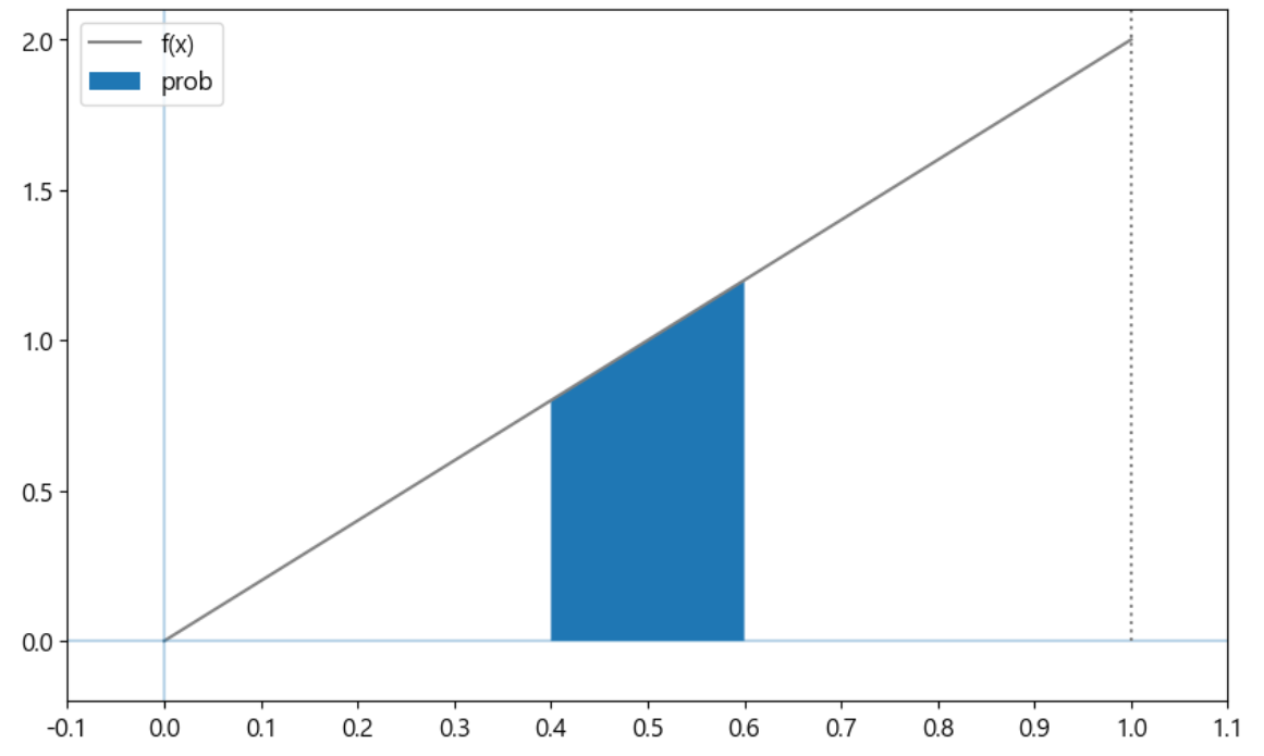
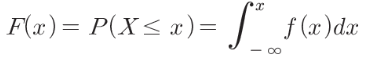
- F(x)의 누적분포함수 구하기
def F(x):
    return integrate.quad(f,-np.inf,x)[0]
ex) 0.4 ≤ X ≤ 0.6 사이 누적값 구하기
F(0.6) - F(0.4)
- 누적분포함수 그래프 그리기
xs = np.linspace(x_range[0], x_range[1], 100)

fig = plt.figure(figsize=(10,6))
ax = fig.add_subplot(111)

ax.plot(xs, [F(x) for x in xs], label = 'F(x)', color = 'gray')
ax.hlines(0,-0.1,1.1,alpha=0.3)
ax.vlines(0,-0.1,1.1,alpha=0.3)
ax.vlines(xs.max(),0,1,linestyles=':',color = 'gray')

ax.set_xticks(np.arange(-0.1,1.2,0.1))
ax.set_xlim(-0.1,1.1)
ax.set_ylim(-0.1,1.1)
ax.legend()

plt.show()
- 확률밀도 함수와 확률분포함수 구하기
1. 확률변수의 변환
- X가 연속형 확률변수
- Y=2X+3 인 Y도 연속형 확률변수
- Y의 확률밀도함수 g(y)
- 확률분포함수 G(y)
y_range = [3,5]

def g(y):
    if y_range[0] <= y <= y_range[1]:
        return (y-3)/2
    else:
        return 0
def G(y):
    return integrate.quad(g,-np.inf,y)[0]
2. 확률밀도함수 & 확률분포함수 그래프 그리기
ys = np.linspace(y_range[0], y_range[1], 100)

fig = plt.figure(figsize=(10,6))
ax = fig.add_subplot(111)

ax.plot(ys, [g(y) for y in ys], label = 'g(y)', color = 'gray')
ax.plot(ys, [G(y) for y in ys], label = 'G(y)', ls = '--', color = 'gray')
ax.hlines(0,2.8,5.2,alpha=0.3)
ax.vlines(ys.max(),0,1,linestyles=':',color = 'gray')

ax.set_xticks(np.arange(2.8,5.2,0.2))
ax.set_xlim(2.8,5.2)
ax.set_ylim(-0.1,1.1)
ax.legend()

plt.show()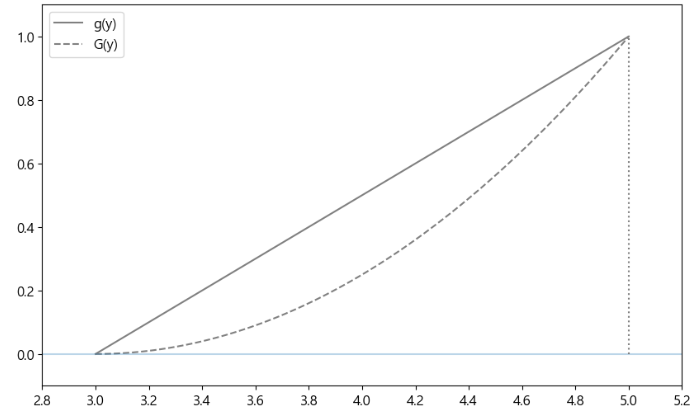
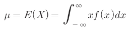
- 연속형 확률변수의 기댓값
1. 기댓값
2. 불공정한 룰렛의 기댓값
def integrand(x):
    return x*f(x)
integrate.quad(integrand,-np.inf,np.inf)[0]
3. 연속형 확률변수의 기댓값
def E(X,g=lambda x:x):
    x_range, f=X
    def integrand(x):
        return g(x)*f(x)
    return integrate.quad(integrand,-np.inf,np.inf)[0]
4. X의 기댓값, Y의 기댓값
E(X) E(Y) = E(X,g=lambda x:2*x+3)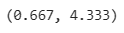
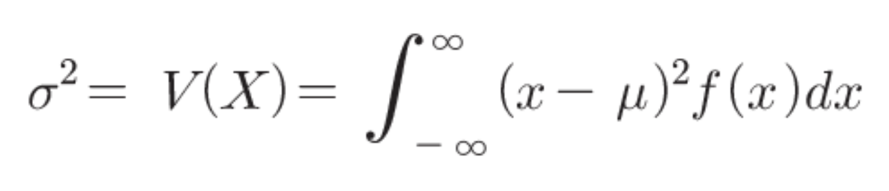
- 연속형 확률변수의 분산
1. 분산
2. 불공정한 룰렛의 분산
mean = E(X)
def integrand(x):
    return (x-mean) **2 *f(x)

integrate.quad(integrand,-np.inf,np.inf)[0]
3. 연속형 확률변수의 분산
def V(X,g=lambda x:x):
    x_range, f=X
    mean = E(X,g)
    def integrand(x):
        return (g(x)-mean) **2 *f(x)
    return integrate.quad(integrand,-np.inf,np.inf)[0]
4. X의 분산, Y의 분산
V(X) V(Y)=V(X,g=lambda x:2*x+3)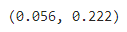
'개념정리 > Python' 카테고리의 다른 글
| ▷ 대표적인 이산형 확률변수 - 베르누이 분포, 이항분포, 기하분포, 포아송분포 (2) | 2023.03.22 |
|---|---|
| ▷ 이산형 확률변수 - 1 · 2차원 이산형 확률변수 (0) | 2023.03.22 |
| ▷ Python 추측 통계의 기본 - 표본추출방법, 확률 분포 (0) | 2023.03.20 |
| ▷ Python 2차원 데이터 정리 - 공분산, 상관계수, 산점도, 회귀직선, 히트맵 (0) | 2023.03.19 |
| ▷ Python 1차원 데이터 정리(PART 3) - 도수분포표, 히스토그램, 상자그림 (0) | 2023.03.18 |


